Vertical Lookup or VLOOKUP – It is one of the most used functions of Microsoft Excel. It is a function to lookup data in a vertically organized table.
It has mainly four components as shown in the below figure:
Lookup_value: The value you want to search for.
Table_array: The table range, which contains both the
lookup value and the result value.
Col_index_num: Column number in the table which
contains the result value.
Range_lookup: FALSE or 0 for an exact match, TRUE or 1 for approximate match.
Let’s see an example of a Simple V lookup formula:
We must find the State where John lives from the Table range
provided to us.
So, Here "John" is our lookup value mentioned in cell “E3”
Our table range is “A1 to B12”
Col_index number is 2, as it’s the 2nd column in
the Table range
Range Lookup = False or 0, which is exact match
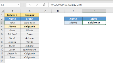
So, to find out the State for John, we will use VLOOKUP
formula as shown in below figure:
Last step is to close the bracket and Press Enter and we can
see the result is displayed as “New York” from the table array range
Lets changed the name to Shawn in Cell "E3" and see if it displays the
State for him.
So, this is how a simple VLOOKUP normally works.
Thank You!


