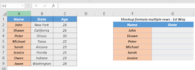
Here I will demonstrate how to get lookup result on multiple rows by entering formula in just a single cell
1st Alternative:
Ctrl + Enter Method:
This is a very simple method. There are 3 Steps involved in it.
Step 1: Highlight all cells starting from G3 till G9, where we need the formula.
The formula will be copied to all selected cells.
1st Alternative method👇
2nd Alternative:
VLOOKUP - Dynamic Array
For Office 365 Only
This method is a feature of Excel Dynamic Array formulas.
The only part which is different from traditional VLOOKUP approach is that , here when we are going to input the lookup value, we will take the whole range, rather then just a single cell.
See in above figure Cell G16 formula is =VLOOKUP(F13:F18,A1:C9,2,0)
Which means we have taken the range of Lookup value instead of just the cell.
So, once this formula is entered, Just press Enter
The formula will spill to the below cells.


